How BEAM works

BEAM stands for Bidirectional Expert-Anchored Model. This page builds the model up step by step: two experts read every residue, their counts become probabilities through a prior, and a single sweep sums over every possible sequence. None of it is needed to use BEAM, but it explains how its answers are computed over every possible sequence rather than estimated by simulation.

Every residue is read twice

Many sequence families are anchored at both ends. A CDR3, the example on this page, is assembled from gene segments: its start is encoded by the V gene and its end by the J gene; the middle is the junction, where nucleotides are added and removed at random. So the start of a CDR3 is best described by counting positions from the front, and the end by counting from the back: the residue three from the end of a CDR3 is constrained by the J gene, whatever the CDR3’s length.

An expert and its window

BEAM reads every sequence with two components, called experts. An expert walks along a sequence one residue at a time, and at each residue it predicts what is there from two things only:

• where it is, counted from its own end of the sequence;
• what it has just read: the $k$ residues before it, its context window. The reference model reads $k = 4$.

Its prediction is a probability for each of the 20 amino acids, learned from the training sequences (below). The forward expert walks from the start, so its window holds the residues before; the backward expert walks from the end, reading the sequence backwards, so its window holds the residues after. Both walk the whole sequence, and they cross in the middle:

Two experts walk a sequence

Loading…

Press Walk to move both experts along CASSLGQGYEQYF, one residue per step: the forward expert (teal) from the start, the backward expert (orange) from the end. Each window frames what its expert looks at: the four residues it has just read (shaded) and the residue it predicts (shown as ? until revealed); dashed tiles lie past the end of the sequence. Each card shows its expert's prediction under the reference model, a probability for each amino acid. Once the residues are revealed, the strip under the sequence keeps the probability each expert gave: the forward expert's above the line, the backward expert's below it.

Both experts are sure of the opening CAS and the closing F, giving each of them 0.89 or more. In the junction between them both are less certain, and they often disagree: at residue 5, L, the forward expert gives 0.25 and the backward expert 0.10; at residue 9, Y, the forward expert gives 0.05, while the backward expert, which has just read EQYF, gives 0.71.

Two experts, one factor

Every residue therefore gets two probabilities, $q_F$ from the forward expert and $q_B$ from the backward expert. BEAM combines them into the residue’s factor, their weighted geometric mean:

$$\psi_i \;=\; q_F^{\,w_F}\; q_B^{\,w_B}, \qquad w_F = w_B = \tfrac{1}{2} \text{ by default.}$$

A geometric mean is high only when both experts find the residue plausible; when one of them objects, the factor falls. So the model knows the conserved start and the conserved end, without being told which V or J genes exist. Change only the last residue of a typical CDR3 from F to W, an ending that is rare in TCRβ CDR3s, and both experts object: the backward expert has rarely seen a sequence end in W, and the forward expert has rarely seen W follow YEQY.

terminal_residue.py

import BEAM

model = BEAM.load_pretrained("human_tcrb_cdr3_aa_foundation")

real = "CASSLGQGYEQYF"
swapped = "CASSLGQGYEQYW"          # the same, with the final F changed to W

print(f"{real}   {model.pseq(real):.3e}")
print(f"{swapped}   {model.pseq(swapped):.3e}")
print(f"ratio: {model.pseq(real) / model.pseq(swapped):,.0f}")

Output

CASSLGQGYEQYF   3.296e-05
CASSLGQGYEQYW   4.304e-12
ratio: 7,656,791

Full program, including the set-up hidden here

Weighing two experts

Loading…

Choose a residue of the sequence: the two experts' windows close in on it, the forward expert's from the left and the backward expert's from the right. The rows are their two predictions for that residue and, below them, the combined factor ψ for every amino acid. Choose a column to read out its factor, for instance W at the last residue, and move the slider to change the weights; at either end of the slider, one expert alone decides. The factors need not add up to one: the normaliser, below, takes care of that.

A model is a table of counts

Building a model is counting. Each expert keeps a table with one row for every position, counted from its own end, and every context of the $k$ residues before it in its reading direction; each row records how often each residue came next. The animation counts a small training set of six CDR3s with $k = 2$, so that its rows fit on screen:

Counting a training set

Loading…

Press Count to walk both experts through the training sequences together. At each residue, the forward expert counts it in the row of its position from the start and the two residues before it (teal window), and the backward expert in the row of its position from the end and the two residues after it (orange window). Each card shows that row's counts so far.

An expert’s probability of a residue comes from its row: from the counts where the row was seen often, and from a prior where it was seen rarely or never, as the next section explains.

Sequences the model has never seen

A repertoire contains a vanishing fraction of all possible CDR3s, so a model must say something sensible about sequences it never saw. The longer an expert’s context, the more specific its prediction, but the more rarely that exact context was seen: four given residues at a given position may have been seen thousands of times, a few times, or never. BEAM resolves this with a hierarchical prior: each level’s prediction is a weighted average of what its own context was seen to do and what the next shorter context predicts,

$$P_j(x) \;=\; \lambda_j\,\frac{n_j(x)}{n_j} \;+\; (1 - \lambda_j)\,P_{j-1}(x), \qquad \lambda_j \;=\; \frac{n_j}{n_j + \alpha_j}$$

• $n_j$ is how often the context of $j$ residues was seen at this position, and $n_j(x)$ how often residue $x$ followed it;
• $\lambda_j$ is the weight on those counts. It grows with $n_j$: a context seen far more often than $\alpha_j$ times speaks for itself, and one never seen passes on the shorter context’s prediction unchanged;
• the chain starts from every residue equally likely and climbs from the position alone ($j = 0$) to the full context ($j = k$).

The prior, level by level

Loading…

Choose a sequence, an expert and a residue; the window marks the context. From the bottom up, each level mixes what its context was seen to do (teal) with what the level below predicts (indigo). Its answer (white) lies between the two, closer to the one with more weight, and is handed up to the next level (dashed line); the top row is the expert's probability, the value explain returns. The model is built from 20,000 cells drawn from the reference model. The slider multiplies every strength α: lower values trust thin counts, higher values lean on short contexts. The lower panel shows how likely 5,000 new cells are at each multiple, relative to the best.

This is the right thing to do for four reasons:

• Trust follows the evidence. A context’s counts get weight in proportion to how often it was seen, so a context seen twice cannot overrule a shorter one seen thousands of times.
• Nothing is ruled out. Every residue keeps some probability from the levels below, so a new sequence is less likely, never impossible.
• It is the Bayesian answer. $P_j$ is the posterior mean of the context’s distribution under a Dirichlet prior centred on the shorter context’s prediction, with strength $\alpha_j$.
• The data choose the strengths. BEAM sets each $\alpha_j$ to the value under which its own counts are most probable, their evidence, without holding any data out. New sequences are on average 98% as likely under the strengths it chooses as under the best multiple of them, and the strengths adapt to how much data there is: built from 20,000 cells, the model gives four residues of context a strength of 3.1 million, passing the three-residue prediction through almost unchanged, while the reference model, built from far more sequences, gives the same level a strength of 78.

The result: a plausible new CDR3 gets a moderate probability, a junk string gets a vanishingly small one, and every sequence up to the maximum length is possible.

What a model stores

A model stores counts, not probabilities. That is why two models can be pooled (merged), and why a saved model reloads to exactly the same probabilities. Only the contexts that were observed are stored.

Assembling a probability

A sequence’s probability is the product of its residues’ factors and the probability of its length, divided by a normaliser. For a sequence $s = s_1 \cdots s_L$ of length $L$,

$$P(s) \;=\; \frac{\pi(L)}{Z(L)} \prod_{i=1}^{L} \psi_i$$

• $\pi(L)$ is the probability of the length;
• $\psi_i$ is residue $i$‘s factor, from the two experts;
• $Z(L)$ is the normaliser: the same product of factors summed over every sequence of length $L$, so that, given the length, the probabilities add up to one.

explain returns all of these terms in logs (see Which residues drive a score), and they add up to the model’s own score:

assemble.py

import BEAM

model = BEAM.load_pretrained("human_tcrb_cdr3_aa_foundation")
s = "CASSLGQGYEQYF"
e = model.explain(s)

# ln P(s) = ln pi(L) + sum_i ln psi_i - ln Z(L), with ln psi_i = w_F ln q_F + w_B ln q_B
print(f"length term   ln pi(L)        = {e['log_length_prior']:9.4f}")
print(f"residue terms sum of ln psi_i = {e['combined'].sum():9.4f}")
print(f"normaliser    ln Z(L)         = {e['log_partition']:9.4f}")
print(f"ln P(s), assembled            = {e['log_length_prior'] + e['combined'].sum() - e['log_partition']:9.4f}")
print(f"ln P(s), from log_pseq        = {model.pseq(s, log=True):9.4f}")

Output

length term   ln pi(L)        =   -1.7650
residue terms sum of ln psi_i =  -10.3225
normaliser    ln Z(L)         =   -1.7671
ln P(s), assembled            =  -10.3203
ln P(s), from log_pseq        =  -10.3203

Full program, including the set-up hidden here

Assembling a probability

Loading…

Press Assemble to build the probability of CASSLGQGYEQYF under the reference model, one factor at a time. The axis is a log scale, so each factor below one moves the running value to the right by its size: first the probability of the length, then each residue's factor ψ (the two experts' windows mark the residue), and last the division by the normaliser Z(13), which moves it back to the left. The end point is the sequence's probability, as log_pseq returns it.

Summing over every sequence

The normaliser $Z(L)$ adds up the product of factors of every sequence of length $L$. There are $20^L$ of them, more than $10^{16}$ for a typical CDR3 of 13 residues, so listing them is impossible, and BEAM never does. Each factor depends only on a residue and the $k$ residues around it, so once the start of a sequence is written, everything still to come depends only on its last $k$ residues: its state. All the starts that end in the same state can be added up and carried forward as one number.

BEAM therefore sweeps the positions from start to end, keeping one running total per state. A state’s total is the sum, over the states it can be reached from, of their totals times the factor of the step; after the last position, the totals add up to $Z(L)$. This is a dynamic program over a layered graph, one layer per position. The animation sweeps a small model of DNA sequences with $k = 2$, small enough to draw every state:

One sweep through the layered graph

Loading…

Press Sweep to sweep a model built from ten short DNA sequences of 6 to 11 bases, with k = 2, for length 8. Each column is one position, and each dot a state: the last two residues written (N stands for an unread base), grouped by the residue written last. At each step, every state collects the totals of the five states it can be reached from, each times the factor of the step: the forward expert's factor for the new residue and the backward expert's for the residue two back, which the new residue completes. Dot size is the state's share of its column's total, and line width the share each edge brings. Choose a dot to see its sum. The bars compare the sequences summed so far with the edges walked.

The reference model’s graph for length 13 has 1,608,421 states and 28,968,420 edges, and one sweep through it adds up every one of $20^{13} \approx 8 \times 10^{16}$ sequences.

The same idea gives every other quantity on this site that sums over all sequences: expected numbers of distinct sequences, overlaps, publicness and distances are computed by sweeps through the graph instead of by listing or sampling sequences.

On a model small enough to list every sequence, the total probability can be checked directly:

normalised.py

import itertools
import math
from BEAM import BeamModel
# A small model over sequences of up to 4 residues, so that every one of them
# can be listed: 20 + 20**2 + 20**3 + 20**4 = 168,420 sequences.
model = BeamModel(sequences, order=2, max_length=4)

every = ["".join(t) for L in range(1, 5) for t in itertools.product("ACDEFGHIKLMNPQRSTVWY", repeat=L)]
total = math.fsum(math.exp(v) for v in model.log_pseq_batch(every) if v > -math.inf)
print(f"{len(every):,} sequences, total probability {total:.15f}")

Output

168,420 sequences, total probability 0.999999999999994

Full program, including the set-up hidden here

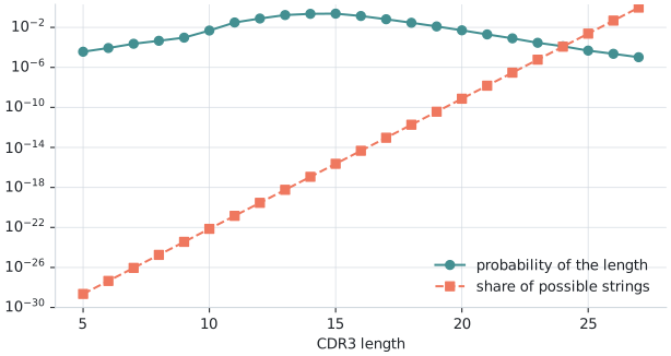
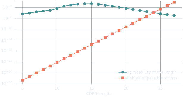
Where the probability lives

Under the reference model, every string of up to 27 amino acids has some probability, but almost all of the probability sits on a tiny fraction of them. By length, most possible strings are long, while most CDR3s are 13 to 16 residues; and within each length, a small share of the strings carries most of the probability.

where_probability_lives.py

import numpy as np
import BEAM

BEAM.set_memory_budget(32 << 30)          # the fine probability grid below needs about 20 GB
model = BEAM.load_pretrained("human_tcrb_cdr3_aa_foundation")

# 1. By length: the model's probability against the share of all possible strings
strings = {L: 20.0 ** L for L in range(1, 28)}
total = sum(strings.values())
print("length   probability   share of possible strings")
for L in range(10, 21, 2):
    print(f"{L:6}   {model.length_distribution.get(L, 0):11.3g}   {strings[L] / total:25.2e}")
print(f"{27:6}   {model.length_distribution.get(27, 0):11.3g}   {strings[27] / total:25.2e}")

# 2. By probability: how much of the probability sits on how few sequences,
#    with every sequence grouped onto a fine grid of probabilities
p, w = model.pseq_analysis().atoms(16384).as_arrays()
order = np.argsort(p)[::-1]
mass = np.cumsum(p[order] * w[order])
support = np.cumsum(w[order]) / w.sum()
for cut in (1e-8, 1e-10, 1e-12):
    k = np.searchsorted(-p[order], -cut, side="right") - 1
    print(f"sequences with P >= {cut:.0e}: {mass[k]:.1%} of the probability, {support[k]:.1e} of the strings")

Output

length   probability   share of possible strings
    10       0.00483                    7.25e-23
    12        0.0768                    2.90e-20
    14         0.225                    1.16e-17
    16         0.137                    4.64e-15
    18        0.0289                    1.86e-12
    20       0.00508                    7.42e-10
    27      1.04e-05                    9.50e-01
sequences with P >= 1e-08: 49.9% of the probability, 5.8e-29 of the strings
sequences with P >= 1e-10: 78.0% of the probability, 3.6e-27 of the strings
sequences with P >= 1e-12: 91.7% of the probability, 1.6e-25 of the strings

Full program, including the set-up hidden here

Strings of 27 residues are 95% of all possible strings, yet the model almost never produces them. And the sequences with probability above $10^{-8}$ carry half of all the probability while making up about $10^{-28}$ of the possible strings: a vanishingly small, highly structured corner of sequence space.

The probability of each length under the reference model against the share of all possible strings of that length.

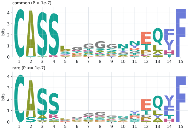
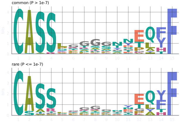
What the model says about each position

At a given length, the probability of each residue at each position is computed over every sequence of that length (positional_marginals), and drawn as a sequence logo it shows the conserved start, the conserved end and the variable junction between them.

Sequence logos of the reference model

Loading…

Choose a CDR3 length to see the probability of each residue at each position, drawn as a sequence logo: letter height is the residue's share of the information at that position. For lengths 13 to 16, switch between the common sequences (probability above 10⁻⁷) and the rare ones.