Comparing groups — cell types, conditions, cohorts

The question: my repertoires fall into groups (cell types, tissues, conditions, patient cohorts). How do the groups differ, which group does a new sequence or sample resemble, and do the samples cluster by group?

The paper asked exactly these questions of real data: clustering mouse repertoires by sorted cell population (CD4, CD8, double negative), comparing naive and memory repertoires within CD4 and CD8, and matching CD4 and CD8 repertoires across two independent studies. The examples here use stand-in groups with known, built-in differences, so that you can see what each method recovers:

• group A: sequences as in the reference population;
• group B: CDR3s tilted towards longer lengths;
• group C: CDR3s enriched for the junction motif PG.

Each stand-in repertoire is a sample of cells from its group’s population. Replace them with your own repertoires and labels.

Group models

Build one model per group from all of its repertoires’ cells pooled together (see Which model do I need?). Each group model can then score any sequence.

Which group does a sequence look like?

Score a sequence under each group’s model: the group under which it is most probable is the one it resembles most, and the difference in log probability says by how much. To assign a whole repertoire, build its model and find the group model nearest to it by distance. (The paper matched CD4 and CD8 repertoires across two studies by the closely related nearest-neighbour rule: each repertoire was assigned the cell type of its nearest repertoire, by distance, among the other study’s repertoires.)

which_group.py

import numpy as np
from BEAM import BeamModel
from BEAM.analytics.distance import compare
# train[g]: all cells of group g's repertoires; new_donor[g]: a repertoire not used to build
groups = "ABC"
models = {g: BeamModel(train[g], order=3) for g in groups}    # one model per group

print("one sequence at a time  (share of a new donor's sequences most probable under each group)")
for true in groups:
    seqs = sorted(set(new_donor[true]))
    scores = np.vstack([models[g].log_pseq_batch(seqs) for g in groups])
    called = scores.argmax(axis=0)
    shares = "  ".join(f"{g}: {np.mean(called == i):.0%}" for i, g in enumerate(groups))
    print(f"  donor from {true}:  {shares}")

print("whole repertoire  (distance from the donor's model to each group's model)")
for true in groups:
    donor = BeamModel(new_donor[true], order=3)
    d = {g: compare(donor, models[g]).distance for g in groups}
    nearest = min(d, key=d.get)
    print(f"  donor from {true}:  " + "  ".join(f"{g}: {d[g]:.4f}" for g in groups) + f"   nearest: {nearest}")

Output

one sequence at a time  (share of a new donor's sequences most probable under each group)
  donor from A:  A: 54%  B: 26%  C: 20%
  donor from B:  A: 32%  B: 53%  C: 15%
  donor from C:  A: 34%  B: 20%  C: 46%
whole repertoire  (distance from the donor's model to each group's model)
  donor from A:  A: 0.1470  B: 0.3689  C: 0.2229   nearest: A
  donor from B:  A: 0.3644  B: 0.1546  C: 0.3643   nearest: B
  donor from C:  A: 0.2237  B: 0.3683  C: 0.1479   nearest: C

Full program, including the set-up hidden here

One sequence carries some evidence; a repertoire carries a lot. Each group’s model is the most probable for about half of its own group’s sequences, against a third by chance: a long CDR3 points to group B, a PG motif to group C. Over a whole repertoire the evidence adds up: the distance from a new donor’s model to each group’s model places every donor with its own group: about 0.15 from its own group’s model, against at least 0.22 from any other.

Assign repertoires by distance

The distance compares two models as whole distributions, length by length and pattern by pattern, so it places a repertoire by what its population looks like, whatever the groups’ diversity. Summing a repertoire’s log probabilities under each group model instead depends on how much of each group’s population its model has seen, which favours less diverse groups. Build group models from similar numbers of cells, so that their distances share one noise floor.

Which group does this sequence look like?

Loading…

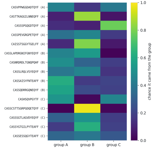
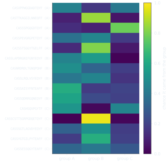
Choose a sequence drawn from one of the three stand-in groups. The bars show its log probability under each group's model; the text gives the resulting chance that it came from each group, with the three groups equally likely beforehand.

Clustering repertoires

Build one model per repertoire, compute the distance between every pair, and cluster. Order 3 makes each comparison take seconds, which matters when there are many pairs; the default order 4 is more detailed.

cluster.py

import itertools
import numpy as np
from scipy.cluster.hierarchy import dendrogram, fcluster, linkage
from scipy.spatial.distance import squareform
from BEAM import BeamModel
from BEAM.analytics.distance import compare
# repertoires: 12 repertoires, 4 from each of groups A, B and C; labels: their groups
models = [BeamModel(cells, order=3) for cells in repertoires]   # order 3: fast for many pairs

n = len(models)
D = np.zeros((n, n))
for i, j in itertools.combinations(range(n), 2):
    D[i, j] = D[j, i] = compare(models[i], models[j]).distance

clusters = fcluster(linkage(squareform(D), "average"), 3, "maxclust")
print("cluster of each repertoire:", "  ".join(f"{g}{k % 4 + 1}:{c}" for k, (g, c) in enumerate(zip(labels, clusters))))

nearest = [labels[int(np.argsort(D[i])[1])] for i in range(n)]
print(f"nearest neighbour from the same group: {np.mean([a == b for a, b in zip(labels, nearest)]):.0%}")

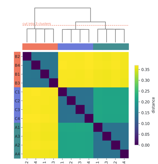
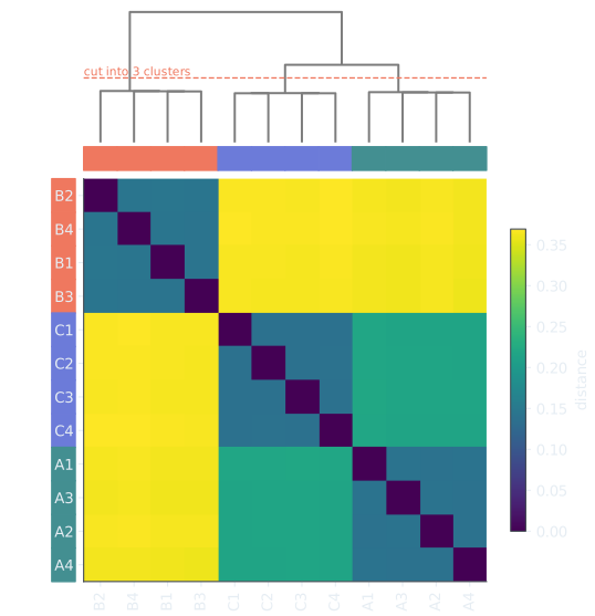
same = [D[i, j] for i, j in itertools.combinations(range(n), 2) if labels[i] == labels[j]]
diff = [D[i, j] for i, j in itertools.combinations(range(n), 2) if labels[i] != labels[j]]
print(f"mean distance within groups: {np.mean(same):.4f}   between groups: {np.mean(diff):.4f}")

Output

cluster of each repertoire: A1:3  A2:3  A3:3  A4:3  B1:1  B2:1  B3:1  B4:1  C1:2  C2:2  C3:2  C4:2
nearest neighbour from the same group: 100%
mean distance within groups: 0.1405   between groups: 0.3156

Full program, including the set-up hidden here

The three clusters are exactly the three groups, every repertoire’s nearest neighbour comes from its own group, and distances between groups (0.32 on average) are more than twice those within them (0.14). Groups A and C, which differ only in how often one motif occurs, are closer to each other than either is to B.

How the repertoires cluster

Loading…

The tree on top is built from the distances alone, without the group labels: repertoires join early when they are close. Cutting it into three clusters (dashed line) gives the three groups, as the colour bands, which show the group each repertoire came from, confirm. The matrix below is the distance between every pair, in the tree's order; dark squares are close pairs. Choose a repertoire's name to see its nearest neighbour and its distance to each group.

Is a difference real?

Repertoires of one group are never identical: each is a finite sample. A difference between groups means something only when it is larger than the differences within groups, which the example above prints. Two useful baselines:

• within-group distances, between repertoires of the same group;
• disjoint samples of one repertoire: split a repertoire’s cells in two and compare the halves.

To compare a property such as “the naive–memory distance is larger in CD8 than in CD4”, compute both distances within each donor and compare them donor by donor, as the paper did (with a sign-flip test over twin families).

Disjoint halves and unequal depths

The distance between two models is never zero, even for two samples of one repertoire: each model sees a finite sample. Two baselines make a distance interpretable, and unequal depths must be removed before comparing:

noise_floor.py

import numpy as np
from BEAM import BeamModel
from BEAM.analytics.distance import compare
# donor_1, donor_2: two repertoires of one population; donor_b: one of another (stand-ins)
def model(cells):
    return BeamModel(cells, order=3)

def distance(x, y):
    return compare(model(x), model(y)).distance

half = 30_000
print(f"two halves of one repertoire:     {distance(donor_1[:half], donor_1[half:]):.4f}")
print(f"two repertoires, one population:  {distance(donor_1[:half], donor_2[:half]):.4f}")
print(f"two repertoires, two populations: {distance(donor_1[:half], donor_b[:half]):.4f}")

# unequal depth: the same comparison with one side ten times smaller
print(f"unequal depth (30,000 vs 3,000 cells), one population: {distance(donor_1[:half], donor_2[:3_000]):.4f}")
print(f"both subsampled to 3,000 cells, one population:         {distance(donor_1[:3_000], donor_2[:3_000]):.4f}")
print(f"both subsampled to 3,000 cells, two populations:        {distance(donor_1[:3_000], donor_b[:3_000]):.4f}")

Output

two halves of one repertoire:     0.1570
two repertoires, one population:  0.1575
two repertoires, two populations: 0.3701
unequal depth (30,000 vs 3,000 cells), one population: 0.2582
both subsampled to 3,000 cells, one population:         0.2564
both subsampled to 3,000 cells, two populations:        0.4309

Full program, including the set-up hidden here

Two halves of one repertoire and two repertoires of one population are equally far apart: that is the noise floor at this depth, and a different population is more than twice as far. The floor depends on depth, and the smaller sample sets it: comparing 30,000 cells with 3,000 gives about the distance between two samples of 3,000, well above the floor at 30,000. So a distance involving a small sample cannot be compared with distances between large ones; compare repertoires at matched depths, each against the floor at that depth.

Which patterns make the groups differ?

Compare two group models with compare to see whether lengths or local patterns drive the difference, and which patterns: see How different are two repertoires?.

What the paper showed with real repertoires

The stand-ins above show the methods. The paper applied them to real data:

• Clustering by cell population. 67 of 69 mouse repertoires clustered with their sorted CD4, CD8 or double-negative population.
• Comparing groups within donors. In all 10 donors from five twin families, naive and memory repertoires were further apart in CD8 than in CD4 T cells, and at 250 clone records per sample these distances exceeded those between disjoint samples of the same repertoire. Separation also held at unequal depths (Supplementary Fig. S8).
• Matching cell types across studies. With references taken entirely from the other study, the nearest repertoire had the same cell type (CD4 or CD8) for 98.9% and 99.2% of queries from two independent studies (30 and 22 people, 1,000 sequences per repertoire).
• The same person over time. In a longitudinal study of two donors, every one of 72 repertoires had its nearest neighbour in the same donor (Supplementary Fig. S10).
• Sensitivity to controlled changes. In simulated repertoires, the distance responded to changed junctional insertions, D-gene trimming and implanted motifs (Supplementary Fig. S9).
• Discovering patterns. Five overlapping length-15 windows, chosen from 12 mice, were enriched in double-negative T cells in all 11 mice held back for validation.

Pitfalls

• Match the depth. Smaller repertoires give noisier models and larger distances. Compare repertoires of similar size, or subsample to a common number of cells first.
• Choose the weighting deliberately. Weighting by abundance lets a few expanded clones dominate a repertoire’s model; counting each distinct sequence once compares sequence composition. See Abundance or unique sequences?
• Same settings for every model. Distances need the same alphabet and order for all models.
• A group model hides variation within the group. Use per-repertoire models when the spread between members matters.