How different are two repertoires, and why?

The question: how different are these two repertoires, and in what way?

Build a model from each repertoire and compare the models. compare gives the distance between them, computed from the models over every possible sequence rather than from the sequences each sample happened to contain, and splits it into parts that say where the difference lies:

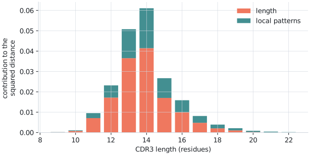
• a part due to different length distributions, for example one repertoire having longer CDR3s;
• a part due to different local patterns: short stretches of sequence that are more common at a given length and position in one repertoire than in the other.

The parts add up exactly to the (squared) distance, so the split is an accounting, not an approximation.

The examples on this page use stand-in repertoires drawn from the reference model, so that the answer is known: two samples of the same population, and one sample from a population shifted towards longer CDR3s and the …NEQFF ending.

A baseline: two samples of one population

Two repertoires of finite size never have identical models, even from the same population. The distance between two such samples is the noise floor against which a real difference stands out.

same_population.py

import BEAM
from BEAM import BeamModel
from BEAM.analytics.distance import compare

# donor_a, donor_a2: two samples of 50,000 cells from the same population
result = compare(donor_a, donor_a2)
print(f"distance: {result.distance:.4f}")
print(f"from lengths: {result.length_squared_distance / result.squared_distance:.1%}"
      f"   from local patterns: {result.pattern_squared_distance / result.squared_distance:.1%}")

Output

distance: 0.1699
from lengths: 0.5%   from local patterns: 99.5%

Full program, including the set-up hidden here

Two different populations

different.py

import BEAM
from BEAM import BeamModel
from BEAM.analytics.distance import compare

# donor_a: as above; donor_b: a repertoire with longer CDR3s and more ...NEQFF endings
result = compare(donor_a, donor_b, top_k=200)
print(f"distance: {result.distance:.4f}")
print(f"from lengths: {result.length_squared_distance / result.squared_distance:.1%}"
      f"   from local patterns: {result.pattern_squared_distance / result.squared_distance:.1%}")

print("\nlocal patterns that differ most (probability given the length):")
print("length  position  pattern   donor A   donor B")
for p in result.patterns[:6]:
    print(f"{p.length:6}  {p.start:8}  {p.word:8}  {p.conditional_p:8.4f}  {p.conditional_q:8.4f}")

print("\noverlapping patterns grouped:")
for g in result.group_overlaps().groups[:4]:
    print(f"  length {g.length}, positions {g.start}-{g.end - 1}: {g.consensus}  "
          f"(more common in donor {'A' if g.direction == 'p' else 'B'})")

Output

distance: 0.4523
from lengths: 67.8%   from local patterns: 32.2%

local patterns that differ most (probability given the length):
length  position  pattern   donor A   donor B
    14         9  NEQFF       0.0795    0.6922
    13         8  NEQFF       0.0646    0.6244
    14         8  YNEQF       0.0398    0.3687
    13         7  YNEQF       0.0275    0.3061
    12         7  NEQFF       0.0533    0.4976
    14         9  TEAFF       0.0954    0.0018

overlapping patterns grouped:
  length 14, positions 5-13: GSSYNEQFF  (more common in donor B)
  length 13, positions 5-12: SSYNEQFF  (more common in donor B)
  length 12, positions 4-11: SSYNEQFF  (more common in donor B)
  length 14, positions 7-13: GNTEAFF  (more common in donor A)

Full program, including the set-up hidden here

The distance, 0.45, is well above the noise floor of 0.17, and the split says why: two thirds of it comes from the different length distributions, and the strongest local patterns point straight at the …NEQFF ending that was made more common.

What the distance is made of

The distance compares the two models at two levels: how often each sequence length occurs, and, within each length, how often each short stretch of sequence (a word of $w$ residues, $w = 5$ at the default order) occurs at each position (a window). Its square is a sum of non-negative terms, one level inside the next:

$$D^2 \;=\; \underbrace{\tfrac12 \sum_L \Big(\sqrt{\pi_A(L)} - \sqrt{\pi_B(L)}\Big)^2}_{\text{length part}} \;+\; \underbrace{\sum_L \sqrt{\pi_A(L)\,\pi_B(L)}\;\frac{1}{V_L} \sum_{v=1}^{V_L} h^2\big(P_A^{(L,v)}, P_B^{(L,v)}\big)}_{\text{pattern part}}$$

• $\pi_A(L)$ and $\pi_B(L)$ are the two models’ probabilities of length $L$;
• $P_A^{(L,v)}(y)$ is model A’s probability of word $y$ in window $v$, among sequences of length $L$, computed over every possible sequence of that length; there are $V_L$ windows at length $L$;
• $h^2(P, Q) = \tfrac12 \sum_y \big(\sqrt{P(y)} - \sqrt{Q(y)}\big)^2$ is the squared Hellinger distance between two distributions: 0 when they agree, 1 when they share nothing.

$D$ is the Hellinger distance between the two models’ joint distributions of length, window and word, so it lies between 0 and 1, is symmetric, and obeys the triangle inequality. Walk through it level by level, and choose any window to see the words behind it:

Anatomy of a distance

Loading…

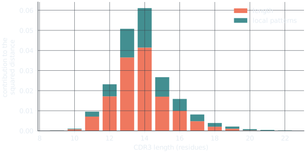
The bar at the top is D² split into its length part (orange) and its pattern part (teal). Step 1 shows the two length distributions and each length's term; step 2 shows every window's share of the pattern part; step 3 shows the words of the chosen window, with one word's term worked out from the formula; step 4 adds everything up. Each step shows the attribute of compare's result that holds its numbers.

Every part, from compare

compare returns every level of the sum, so the analysis above can be run on any pair of models:

parts.py

from collections import Counter
import BEAM
from BEAM import BeamModel
from BEAM.analytics.distance import compare

r = compare(donor_a, donor_b, top_k=5000)

# The squared distance is the length part plus the pattern part
print(f"D^2 = {r.squared_distance:.6f}   (D = {r.distance:.4f})")
print(f"  length part  r.length_squared_distance   = {r.length_squared_distance:.6f}")
print(f"  pattern part r.pattern_squared_distance  = {r.pattern_squared_distance:.6f}")

# Each part, length by length: r.lengths
print(f"  sum of x.contribution over r.lengths         = {sum(x.contribution for x in r.lengths):.6f}")
print(f"  sum of x.pattern_contribution over r.lengths = {sum(x.pattern_contribution for x in r.lengths):.6f}")

# The pattern part, window by window: r.windows (one per length and start)
print(f"  sum of w.contribution over r.windows         = {sum(w.contribution for w in r.windows):.6f}")

# Word by word: r.patterns holds the strongest; r.remainder the rest
print(f"  listed words {r.reported_pattern_squared_distance:.6f} + remainder {r.remainder:.6f}")

# One word's term, by hand: sqrt(pi_A pi_B) (sqrt(p) - sqrt(q))^2 / (2 V_L)
w = r.patterns[0]
L = next(x for x in r.lengths if x.length == w.length)
V = Counter(x.length for x in r.windows)[w.length]          # windows at this length
by_hand = (L.p * L.q) ** 0.5 * (w.conditional_p ** 0.5 - w.conditional_q ** 0.5) ** 2 / (2 * V)
print(f"\nstrongest word: {w.word} at length {w.length}, positions {w.start}-{w.end - 1}")
print(f"  pi_A = {L.p:.4f}  pi_B = {L.q:.4f}  p = {w.conditional_p:.4f}  q = {w.conditional_q:.4f}  V = {V}")
print(f"  by hand {by_hand:.6f}   w.contribution {w.contribution:.6f}")

Output

D^2 = 0.204619   (D = 0.4523)
  length part  r.length_squared_distance   = 0.138776
  pattern part r.pattern_squared_distance  = 0.065843
  sum of x.contribution over r.lengths         = 0.138776
  sum of x.pattern_contribution over r.lengths = 0.065843
  sum of w.contribution over r.windows         = 0.065843
  listed words 0.025204 + remainder 0.040639

strongest word: NEQFF at length 14, positions 9-13
  pi_A = 0.2237  pi_B = 0.0343  p = 0.0795  q = 0.6922  V = 10
  by hand 0.001325   w.contribution 0.001325

Full program, including the set-up hidden here

Each level adds up to the one above it: the lengths’ terms to the two parts, the windows to each length’s pattern term, and the words to their window. The strongest word’s term, worked out by hand from the formula, matches the one compare returns. top_k sets how many words are listed, strongest first; remainder holds the rest, so nothing is left out of the total.

Reading the patterns

Each pattern is a short stretch of sequence at a given length and position, with its probability in each repertoire given the length. Conditioning on length keeps the two parts separate: a pattern term measures a difference in sequence content, not a consequence of different lengths. group_overlaps() joins overlapping patterns into longer motifs, which are easier to read.

Pitfalls

• Compare against a baseline. A distance means little on its own; compare it with the distance between samples of similar size from one population, or between replicates.
• Repertoire size matters. Models of small repertoires are noisier, so their distances are larger. Compare repertoires of similar sizes, or subsample to a common size.
• Same settings. Both models must have the same alphabet and order.
• Comparing takes about 40 seconds for models of the default order 4, on a 16-core machine and whatever the repertoires’ size, and about 3 seconds at order 3, which suits comparing many pairs.