How public is a sequence?

The question: in a cohort of people, how many would I expect to carry this sequence in their sampled repertoire?

A sequence is public when it appears in many people. How many depends on two things: how common the sequence is in the population, which is its probability under the model, and how deeply each person was sampled. PublicnessModel combines them: the mean and variance in closed form, and the full distribution by an accurate numerical inversion.

Expected carriers

Describe the cohort by the depth of each person’s sample, then ask about a sequence’s probability.

one_sequence.py

import math
import BEAM
from BEAM import PublicnessModel

model = BEAM.load_pretrained("human_tcrb_cdr3_aa_foundation")
cohort = PublicnessModel([50_000] * 100)      # 100 people, 50,000 cells sampled from each

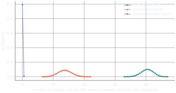
for cdr3 in ["CASSLGQGYEQYF", "CASSLGQGAYNEQFF", "CASSPRDRGLAGGYNEQFF"]:
    mean, variance = cohort.moments(model.pseq(cdr3))
    print(f"{cdr3:20} expected carriers {mean:6.2f} ± {math.sqrt(variance):.2f}")

Output

CASSLGQGYEQYF        expected carriers  80.75 ± 3.94
CASSLGQGAYNEQFF      expected carriers  27.51 ± 4.47
CASSPRDRGLAGGYNEQFF  expected carriers   0.01 ± 0.09

Full program, including the set-up hidden here

moments returns the mean and variance of the number of carriers. The most common of the three sequences is expected in about 81 of the 100 people; the rarest in almost nobody.

The whole distribution

The mean is not the whole story: pmf gives the probability that exactly 0, 1, 2, … people carry the sequence.

distribution.py

import numpy as np
import BEAM
from BEAM import PublicnessModel

model = BEAM.load_pretrained("human_tcrb_cdr3_aa_foundation")
cohort = PublicnessModel([50_000] * 100)

pmf = cohort.pmf(model.pseq("CASSLGQGAYNEQFF"))    # P(exactly k carriers), k = 0..100
print(f"P(nobody carries it)     {pmf[0]:.3f}")
print(f"P(1 to 5 people)         {pmf[1:6].sum():.3f}")
print(f"P(more than 5 people)    {pmf[6:].sum():.3f}")
print(f"most likely: {np.argmax(pmf)} people")

Output

P(nobody carries it)     0.000
P(1 to 5 people)         0.000
P(more than 5 people)    1.000
most likely: 27 people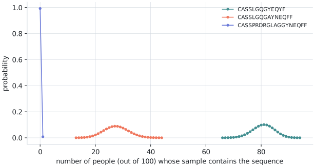

Full program, including the set-up hidden here

How many of 100 people, each sampled to 50,000 cells, carry three sequences of different probability.

Explore publicness

Loading…

Choose a cohort size, a sampling depth and a sequence, or set any sequence probability with the slider. The bars show the probability that each number of people carries the sequence, computed from the reference model.

Cohorts sampled to different depths

Real cohorts mix shallow and deep samples. Give each person’s depth:

unequal.py

import BEAM
from BEAM import PublicnessModel

model = BEAM.load_pretrained("human_tcrb_cdr3_aa_foundation")

# 20 people sampled to 10,000 cells, 50 to 100,000 and 30 to 1,000,000
depths = [10_000] * 20 + [100_000] * 50 + [1_000_000] * 30
cohort = PublicnessModel(depths)

mean, variance = cohort.moments(model.pseq("CASSLGQGAYNEQFF"))
print(f"{cohort.n_repertoires} people, expected carriers {mean:.1f}")

Output

100 people, expected carriers 54.9

Full program, including the set-up hidden here

To stay fast, people of similar depth are grouped into at most 64 groups, each represented by one depth. With 64 or fewer distinct depths, as here, nothing is grouped. With more, the result is a close approximation; cohort.depth_spread gives the widest ratio of depths within a group (1.0 means no grouping), and PublicnessModel(depths, depth_bins=len(set(depths))) avoids grouping altogether.

The most public sequences of a repertoire

moments takes many probabilities at once, so a whole repertoire can be ranked by how public its sequences are expected to be:

rank.py

import numpy as np
import BEAM
from BEAM import PublicnessModel

model = BEAM.load_pretrained("human_tcrb_cdr3_aa_foundation")
# repertoire: the distinct CDR3s of one sample
cohort = PublicnessModel([100_000] * 100)

probabilities = np.exp(model.log_pseq_batch(repertoire))
expected, _ = cohort.moments(probabilities)          # one call for the whole list

order = np.argsort(expected)[::-1]
print("most public sequences of this sample (expected carriers out of 100):")
for i in order[:5]:
    print(f"  {repertoire[i]:18} {expected[i]:5.1f}")
print(f"expected in fewer than one person: {np.mean(expected < 1):.0%} of its sequences")

Output

most public sequences of this sample (expected carriers out of 100):
  CASSPQRNTEAFF      100.0
  CASSQSPGGTQYF      100.0
  CASSQSPGGIQYF      100.0
  CASSALLGSASTQYF    100.0
  CASSLVPEAYNEQFF    100.0
expected in fewer than one person: 71% of its sequences

Full program, including the set-up hidden here

At this depth the most common sequences are expected in all 100 people, while 71% of this sample’s sequences are expected in fewer than one person: most of any repertoire is private. The sequences at the top are the ones a cohort study would see again and again.

The publicness of a whole cohort

Instead of one sequence at a time, ask about every sequence at once: how many sequences are expected to be carried by exactly 1, 2, …, all of the people in a cohort. This is the cohort’s publicness spectrum. BEAM computes it over every sequence the model can produce, grouped onto a fine grid of probabilities (pseq_analysis().atoms). The example’s grid of 16,384 values agrees with the grid-free counts of distinct and private sequences to within 3 × 10⁻⁵; a grid of 4,096 values needs about a third of the memory and stays within about 1.5%.

spectrum.py

import numpy as np
import BEAM
from BEAM import PublicnessModel
from BEAM.analytics.exact_occupancy import ExactOccupancy

BEAM.set_memory_budget(32 << 30)       # a fine probability grid needs about 20 GB
model = BEAM.load_pretrained("human_tcrb_cdr3_aa_foundation")

# Every sequence the model can produce, grouped onto a fine grid of probabilities
p, w = model.pseq_analysis().atoms(16384).as_arrays()
cohort = PublicnessModel([100_000] * 100)             # 100 people, 100,000 cells each

counts = cohort.expected_counts(p, w)["expected_counts"]   # [k]: sequences in exactly k people
seen = counts[1:].sum()
print(f"distinct sequences in the cohort: {seen:,.0f}")
print(f"private (in one person):          {counts[1]:,.0f}  ({counts[1] / seen:.1%})")
for k in (2, 5, 10, 50, 100):
    print(f"in exactly {k:3} people:            {counts[k]:,.1f}")

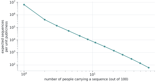
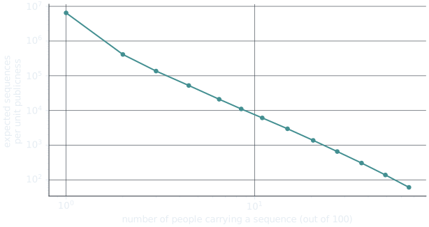
# The grid is an approximation; check it against the grid-free calculation
direct = ExactOccupancy(model).equal_depth_cohort(100_000, 100)
print(f"grid-free: {direct['seen'].value:,.0f} distinct, {direct['private'].value:,.0f} private "
      f"(grid within {abs(seen / direct['seen'].value - 1):.1e} and "
      f"{abs(counts[1] / direct['private'].value - 1):.1e})")

Output

distinct sequences in the cohort: 7,232,357
private (in one person):          6,463,037  (89.4%)
in exactly   2 people:            410,436.8
in exactly   5 people:            38,443.4
in exactly  10 people:            7,463.3
in exactly  50 people:            130.5
in exactly 100 people:            38.6
grid-free: 7,232,134 distinct, 6,462,810 private (grid within 3.1e-05 and 3.5e-05)

Full program, including the set-up hidden here

Of the 7.2 million distinct sequences expected across 100 people, 89% are private to one person, and the counts fall steadily with publicness, approximately as a power law, as in the paper’s predicted spectra. About 39 sequences are expected in all 100 people: common enough that almost everyone carries them, they collect at that boundary, so the plots below leave the top bin out, as the paper’s figure does.

The expected publicness spectrum of 100 people sampled to 100,000 cells each, under the reference model, averaged over log-spaced bins of publicness; the top bin, where sequences in nearly everyone collect, is left out.

The publicness spectrum

Loading…

Choose a cohort size and a sampling depth. Each dot is the expected number of sequences carried by that many people, averaged over log-spaced bins of publicness as in the paper's figure; the top bin, where sequences in nearly everyone collect, is left out. Larger cohorts extend the spectrum to higher publicness; deeper sampling raises it at every level.

How private is each donor?

In a cohort of unequal depths, each person’s expected share of private sequences differs: a deeply sampled donor has more rare sequences that nobody else has. private_at_depth gives each donor’s expected distinct and private counts:

per_donor.py

import numpy as np
import BEAM
from BEAM.analytics.exact_occupancy import ExactOccupancy

model = BEAM.load_pretrained("human_tcrb_cdr3_aa_foundation")
occupancy = ExactOccupancy(model)

depths = np.logspace(4, 6, 10)            # ten donors, 10,000 to 1,000,000 cells
result = occupancy.private_at_depth(depths, total_depth=depths.sum())

print("   cells   distinct   private to this donor")
for d, n, priv in zip(depths, result["distinct"], result["private"]):
    print(f"{d:9,.0f}  {n.value:9,.0f}   {priv.value / n.value:8.1%}")

Output

   cells   distinct   private to this donor
   10,000      9,943      76.2%
   16,681     16,538      76.5%
   27,826     27,471      76.8%
   46,416     45,548      77.3%
   77,426     75,333      78.0%
  129,155    124,204      79.0%
  215,443    204,015      80.4%
  359,381    333,676      82.3%
  599,484    543,171      84.8%
1,000,000    879,776      88.2%

Full program, including the set-up hidden here

The shallowest donors are expected to have about 76% private sequences and the deepest about 88%: deeper samples reach further into the rare sequences that nobody else carries.

This is the baseline the paper compared real donors with: observed private fractions varied between donors more than sampling from one shared distribution produces, so something beyond sampling, biological or technical, differs between them.

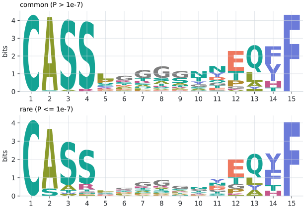
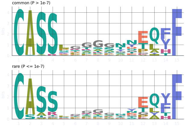
What public sequences look like

Sequence logos of the common and the rare sequences of one length show what probable, and therefore public, sequences look like: common sequences are more constrained. (The paper’s logos, split by expected publicness rather than probability, show the constraint arising first at the start of the CDR3 and then through the junction.)

logos.py

import BEAM

BEAM.set_memory_budget(16 << 30)          # these logos need about 6 GB
model = BEAM.load_pretrained("human_tcrb_cdr3_aa_foundation")

common = model.insights.logo(15, pseq_above=1e-7)   # length-15 sequences with P > 1e-7
rare = model.insights.logo(15, pseq_below=1e-7)     # and the rest
print(f"common: {common.fraction:.1%} of the probability at length 15, consensus {common.consensus_sequence}")
print(f"rare:   {rare.fraction:.1%} of the probability at length 15, consensus {rare.consensus_sequence}")
print(f"information, common vs rare: {common.information_bits.sum():.1f} vs {rare.information_bits.sum():.1f} bits")

Output

common: 25.1% of the probability at length 15, consensus CASSLGGGGNNEQFF
rare:   74.9% of the probability at length 15, consensus CASSLGGGGNYEQYF
information, common vs rare: 37.0 vs 29.4 bits

Full program, including the set-up hidden here

At length 15, the common sequences carry a quarter of the probability and 37 bits of information, against 29 bits for the rare ones: common sequences are more predictable at almost every position.

Sequence logos of length-15 CDR3s under the reference model: sequences with probability above 10⁻⁷ (top) and the rest (bottom).

Pitfalls

• This is the expectation from probability alone. Sharing in real cohorts also comes from shared HLA types and shared exposures, such as a common virus. A sequence carried by many more people than expected is exactly what such an effect looks like, which is what makes the expectation useful.
• Depth is the number of cells sampled per person, not the number of distinct sequences observed.
• The population matters. Under the reference model, probabilities describe a broad aggregate of published repertoires. A cohort that differs from it (another species, another chain, a sorted subset) needs a model of its own population.